长治市网站建设_网站建设公司_Spring_seo优化
主要通过以下9个方面来了解协程的原理:
目录
1、为什么使用协程
1.3、协程的适用场景
2、协程的原语操作
3、协程的切换
3.1、汇编实现
4.协程的运行流程
5.协程的结构体定义(我们其实可以参照线程或者进程的状态来设计)
5.1、多状态集合设计
6.协程的调度策略
7.协程调度器如何定义
8、多核模式
9、性能测试
为什么要有协程?协程解决了什么问题?
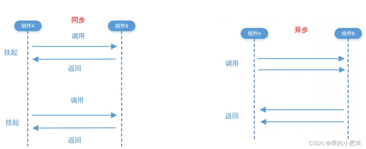
关于协程,我们经常看到这样的话:同步的编程方式,异步的性能。那么什么是同步,什么是异步呢?
同步与异步
同步和异步,是形容两者之间的关系。两者在一个流程内,就是同步;两者不在一个流程内,就是异步。
我们这里说的同步和异步,是指io同步操作和io异步操作。
还有一个容易与io异步操作混淆的概念,异步io,就是指有io数据的时候,直接callback,AIO, 比如boost的asio;
主要差别是在IO事件是否就绪的两种处理方式的区别
方法一:io 同步操作
- 发起请求:等待响应
- 接受响应
对 io 的操作和 epoll_wait 放在同一流程里,需要等待 io 的响应。
优点:sockfd 管理方便,操作逻辑清晰缺点:依赖 io 响应速度,性能差
int handle(int sockfd) {recv(sockfd, rbuffer, length, 0);parser_proto(rbuffer, length);send(sockfd, sbuffer, length, 0);
}
方法二:io 异步操作
handle 函数内部将 sockfd 的操作,push 到线程池中,在 io 数据拷贝阶段可以做其他事。
int thread_cb(int sockfd) {// 此函数是在线程池创建的线程中运行,与 handle 不在一个线程上下文中运行recv(sockfd, rbuffer, length, 0);parser_proto(rbuffer, length);send(sockfd, sbuffer, length, 0);
}
int handle(int sockfd) {//此函数在主线程 main_thread 中运行,在此处之前,确保线程池已经启动。push_thread(sockfd, thread_cb); //将 sockfd 放到其他线程中运行。
}
1、为什么使用协程
从性能方面来看,对于使用异步 io 的线程,存在三个问题:
系统线程占用大量的内存空间
线程切换占用大量的系统时间
为了线程安全,线程间需要加锁保护资源,降低执行的效率
从编程角度来看,无论同步还是异步编程方式,都是基于事件驱动的。事件驱动流程包括注册事件,绑定回调,触发回调,提高了系统的并发。但是由于回调的多层嵌套,使得编程复杂,降低了代码的可维护性。
在资源有限的前提下,高性能服务需要解决的问题有:
减少线程的重复高频创建:线程池
尽量避免线程的阻塞
Reactor + 非阻塞回调:解决问题的能力有限
响应式编程:容易陷入回调地狱,割裂业务逻辑
协程:将同 io 转成异步 io
提升代码的可维护与可理解性:减少回调函数,减少回调链深度
而协程的出现,可以很好地解决上述问题。
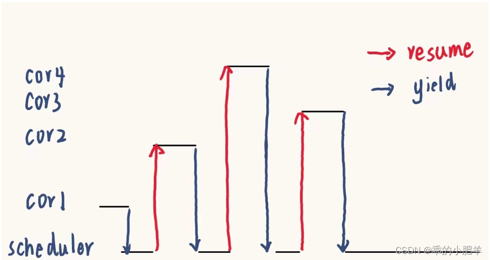
协程运行在线程之上。当一个协程调用阻塞 io,主动让出 cpu ( yield 原语) ,让另一个协程运行在当前线程之上( resume 原语)。协程没有增加线程数量,只是在线程的基础上通过分时复用的方式运行多个协程,降低了系统内存。而且协程的切换在用户态完成,减少了系统切换开销。
综上所述,协程的优势体现在:
消耗系统资源和切换代价更小
协程可以实现无锁编程
简化了异步编程,可以达到以同步的编程方式实现异步的性能。
1.3、协程的适用场景
协程适用于 I/O 密集型业务,线程切换频繁。其他情况,性能不会有太大的提升。
2、协程的原语操作
yield: 协程主动让出CPU给调度器。时机:业务提交 -> epoll_wait
resume: 调度器恢复协程的运行权。时机:epoll_wait -> 业务处理
resume 和 yield 是两个可逆的原子操作。
io 异步操作函数执行流程如下:
将 sockfd 添加到 epoll 管理
由协程上下文 yield 到调度器的上下文
调度器获取下一个协程上下文,resume 新的协程

1.commit完后,switch --> epoll_wait 是 yield (让出(将当前协程从寄存器里让出)操作到wait下等待io就绪,如果IO就绪那么使用resume操作,在将当前协程让出后,把新的协程交换到cpu上运行(寄存器上))
2.epoll_wait --> io处理流程 是 resume (恢复操作)
yield 与 resume 是一个switch操作(三种实现方式):
1.longjump/setjump
2.ucontext
3.汇编实现
3、协程的切换
协程的上下文如何进行切换?现有的 C++ 协程库均基于两种方案
汇编实现:libco,Boost.context
OS 提供的 API :
phxrpc:基于 ucontext / Boost.context 的上下文切换
libmill:基于 setjump/longjump 的协程切换
一般来说,基于汇编的上下文切换要比采用系统调用的切换更加高效
3.1、汇编实现
x86-64有16个64位寄存器,分别是:%rax,%rbx,%rcx,%rdx,%rdi,%rsi,%rbp,%rsp,%r8,%r9,%r10,%r11,%r12,%r13,%r14,%r15。
%rax: Return value, 作为函数返回值使用。
%rsp: Stack pointer,栈指针,栈顶指针,指向栈顶
%rbp: Base pointer,基址指针,栈桢(栈底)指针 Frame pointer,指向栈的底部
%rdi,%rsi,%rdx,%rcx,%r8,%r9: 用作函数参数,依次对应第1, …, 6参数
%rbx,%r12,%r13,%r14,%r15: Caller saved,被调用者保护寄存器(易失性寄存器),程序调用过程中寄存器的值不需要保存。如果要保存,则调用者负责压栈。
%r10,%r11: Callee-owned,调用者保护寄存器(非易失性寄存器)。程序调用过程中,需要保存,不能覆盖。被调用寄存器先保存值然后再调用,调用结束后恢复调用前的值。
%rip: Instruction pointer, 相当于PC指针指向当前的指令地址,指向下一条要执行的指令
协程上下文切换,就是先将 cpu 寄存器的值暂时保存到 cur_ctx,再将即将运行的协程的上下文 new_ctx 的值 mov 到相对应的 cpu 寄存器上,完成切换。
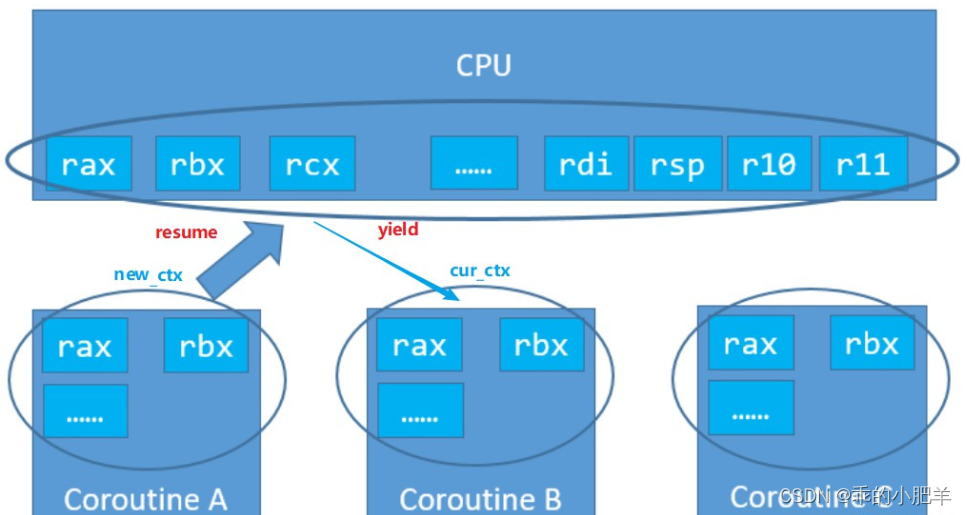
切换函数 _switch 的定义
/*** @brief switch实现协程切换,保存cpu寄存器的值到cur_ctx,加载new_ctx上下文到cpu寄存器* @param new_ctx: 对应寄存器rdi,即将运行协程的上下文,加载它的上下文到cpu寄存器* @param cur_ctx: 对应寄存器rsi,正在运行协程的上下文,保存cpu寄存器到它的上下文 * @return int */
int _switch(nty_cpu_ctx *new_ctx, nty_cpu_ctx *cur_ctx);
//
__asm__ (
"    .text                                  \n"
"       .p2align 4,,15                                   \n"
".globl _switch                                          \n"
".globl __switch                                         \n"
"_switch:                                                \n"
"__switch:                                               \n"
"       movq %rsp, 0(%rsi)      # save stack_pointer     \n"
"       movq %rbp, 8(%rsi)      # save frame_pointer     \n"
"       movq (%rsp), %rax       # save insn_pointer      \n"
"       movq %rax, 16(%rsi)                              \n"
"       movq %rbx, 24(%rsi)     # save rbx,r12-r15       \n"
"       movq %r12, 32(%rsi)                              \n"
"       movq %r13, 40(%rsi)                              \n"
"       movq %r14, 48(%rsi)                              \n"
"       movq %r15, 56(%rsi)                              \n"
"       movq 56(%rdi), %r15                              \n"
"       movq 48(%rdi), %r14                              \n"
"       movq 40(%rdi), %r13     # restore rbx,r12-r15    \n"
"       movq 32(%rdi), %r12                              \n"
"       movq 24(%rdi), %rbx                              \n"
"       movq 8(%rdi), %rbp      # restore frame_pointer  \n"
"       movq 0(%rdi), %rsp      # restore stack_pointer  \n"
"       movq 16(%rdi), %rax     # restore insn_pointer   \n"
"       movq %rax, (%rsp)                                \n"
"       ret                                              \n"
);
nty_cpu_ctx 结构体,存储寄存器的值
// x86 寄存器列表,每个寄存器8字节
typedef struct _nty_cpu_ctx {void *esp; void *ebp;void *eip;void *edi;void *esi;void *ebx;void *r1;void *r2;void *r3;void *r4;void *r5;
} nty_cpu_ctx;
4.协程的运行流程
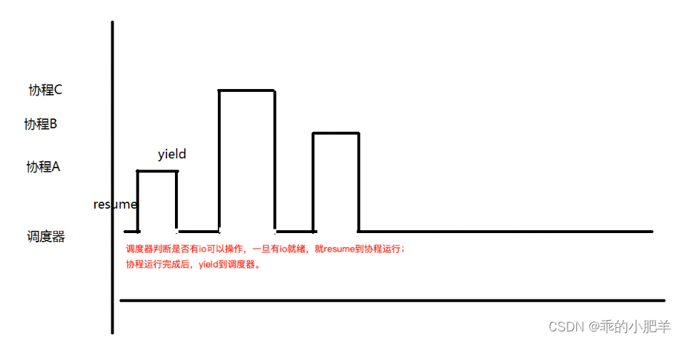
协程中遇到io操作,就加入到epoll里面,yield,将CPU让出,回到调度器,调度器进行调度,决定哪个协程运行。
一个fd对应一个协程的设计方法,是不是最优的?能不能设计成多分fd对应一个协程?
对于网络框架,一个fd对应一个协程是一个很好的方案;
如果是对界面刷新或者磁盘文件操作,就不是很合适。
比如A协程 recv,如果该fd io已经准备就绪了,这时候yield,调度器会调度其他协程运行,可能调度几百几千个其他协程,最后再回到A协程进行recv,它的实时性有没有意义?
对于大量io,所有io一起看的话,单个io的实时性是没有意义的。
5.协程的结构体定义(我们其实可以参照线程或者进程的状态来设计)
//这里我们就采用比较简单的方式来实现
协程数据结构设计分为两部分
- 运行体 R:包含运行状态(就绪,睡眠,等待),运行体回调函数,回调参数,栈指针,栈大小,当前运行体
- 调度器 S:包含执行集合(就绪,睡眠,等待)
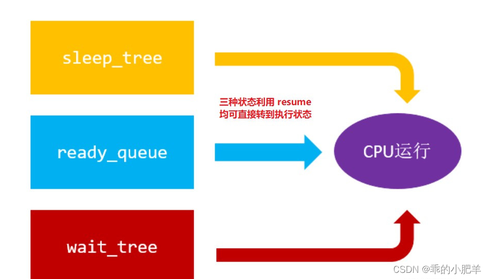
5.1、多状态集合设计
新创建的协程,创建完成后,加入到就绪集合,等待调度器的调度;协程在运行完成后,进行 IO 操作,此时 IO 并未准备好,进入等待状态集合;IO 准备就绪,协程开始运行,后续进行 sleep 操作,此时进入到睡眠状态集合。
那么,运行体如何在多状态集合高效切换?三种集合如何设置合理的数据结构?
就绪 (ready) 集合:不设置优先级,所有协程优先级一致,使用队列存储就绪的协程,简称就绪队列 (ready_queue)
睡眠 (sleep) 集合:需要对睡眠时长排序,采用红黑树来存储,简称睡眠树 (sleep_tree)。key 为睡眠时长,value 为对应的协程结点。
等待 (wait) 集合:需要对 IO 等待时间排序,采用红黑树来存储,简称等待树 (wait_tree)。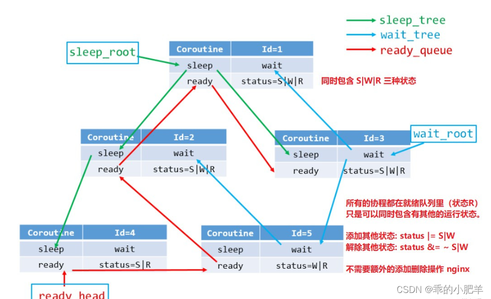
struct coroutine {nty_cpu_ctx ctx; 				    //上下文环境,保存CPU寄存器proc_coroutine func;		  	    // 子过程的回调函数void *arg;						   // 子过程回调函数的参数void *ret;						   // 子过程回调函数的返回值nty_coroutine_status status;	   	 // 运行状态:ready, wait, sleepnty_schedule *sched;				// 调度器uint64_t birth;					    // 创建时间uint64_t id;					    // 协程 idvoid *stack;					  	// 栈空间size_t stack_size;			  	  	 // 栈空间大小RB_ENTRY(_nty_coroutine) sleep_node;	// 睡眠 sleep 树RB_ENTRY(_nty_coroutine) wait_node;		// 等待 wait 树TAILQ_ENTRY(_nty_coroutine) ready_next;	// 就绪 ready 队列
};
我们每个协程有自己独立的栈空间比较好,共享栈的话在编程和处理方面比较麻烦
6.协程的调度策略
协程如何被调度,有两种方案,生产者消费者模式和多状态运行。

while (1) {//遍历睡眠集合,将满足条件的加入到 readynty_coroutine *expired = NULL;while ((expired = sleep_tree_expired(sched)) != NULL) {TAILQ_ADD(&sched->ready, expired);}//遍历等待集合,将满足添加的加入到 readynty_coroutine *wait = NULL;int nready = epoll_wait(sched->epfd, events, EVENT_MAX, 1);for (i = 0;i < nready;i ++) {wait = wait_tree_search(events[i].data.fd);TAILQ_ADD(&sched->ready, wait);}// 使用 resume 恢复 ready 的协程运行权while (!TAILQ_EMPTY(&sched->ready)) {nty_coroutine *ready = TAILQ_POP(sched->ready);resume(ready);}
}
多状态运行
while (1) {//遍历睡眠集合,使用 resume 恢复 expired 的协程运行权nty_coroutine *expired = NULL;while ((expired = sleep_tree_expired(sched)) != NULL) {resume(expired);}//遍历等待集合,使用 resume 恢复 wait 的协程运行权nty_coroutine *wait = NULL;int nready = epoll_wait(sched->epfd, events, EVENT_MAX, 1);for (i = 0;i < nready;i ++) {wait = wait_tree_search(events[i].data.fd);resume(wait);}// 使用 resume 恢复 ready 的协程运行权while (!TAILQ_EMPTY(sched->ready)) {nty_coroutine *ready = TAILQ_POP(sched->ready);resume(ready);}
}
其实我认为是第一种比较好,因为参照线程和进程的状态来实现会更加贴合操作系统运行
7.协程调度器如何定义
每一协程都需要使用的而且可能会不同属性的,就是协程属性(私有)。每一协程都需要的而且数据一致的,就是调度器的属性(公共)。调度器是管理所有协程运行的组件。
// 调度策略
struct scheduler_op {remove_wait();remove_sleep();
};// 调度器,用来管理所有的协程
struct scheduler {int epfd;					struct epoll_event events[];  struct coroutine *cur;   // 当前运行的协程queue_tail(, struct coroutine) ready;  // 指向就绪队列rbtree_root(, struct coroutine) wait;  // 指向等待树rbtree_root(, struct coroutine) sleep; // 指向睡眠树struct scheduler_op *sch_op; //调度策略
};
这么定义好了之后,调度器就可以遍历各个状态的数据结构,然后加一个定时器,将要超时的
协程调度上来,设置当前运行协程是因为调度器需要运行一个协程,如果来新的协程,再把老的协程执行让出操作,新的协程resume操作,交给调度器进行调度
调度器与协程(每个协程对应一个客户端)的运行关系
if (io 是否可写) {connect();
}
else {epoll_ctl(epfd, fd);yield();
}
8、多核模式
一个线程一个调度器,简单,不需要加锁
一个进程一个调度器,简单,不需要加锁
多个线程共用一个调度器,复杂,入队需要加锁
9、性能测试
测试标准
并发量:fd数量、协程的数量,fd数量 == 协程数量
为什么这么说呢,是因为我们当一个客户端连接的是否,事件就绪,如果是读事件中的监听套接字,那么还需要创建一个新的协程将新的fd加入到epoll中,所以每个客户端连接过来,我们都需要创建一个协程来管理当前客户端的fd
所以说fd数量 == 协程数量
每秒接入量:fd -> coroutine_create
断开连接:coroutine_destory